The glycHem data set

The glycHem data set is a small data set of 20 samples of blood tested for glycated hemoglobin with two different methods that can be used to show the merits of Bayesian Deming regression. It is also possible to highlight the power of the Mahalanobis distance (MD) testing compared to the classical testing with confidence intervals (CI).

For non-robust methods, the comparison between the original frequentist Deming regression and the Bayesian method is straightforward.

To evaluate the robust variant instead, it is worth using Passing Bablok’s equivariant (PBequi) regression as a comparison.

All frequentist methods are calculated with the R {mcr} package; Bayesian Deming regression is calculated with the R {rstanbdp} package.

Bayesian deming vs frequentist Deming

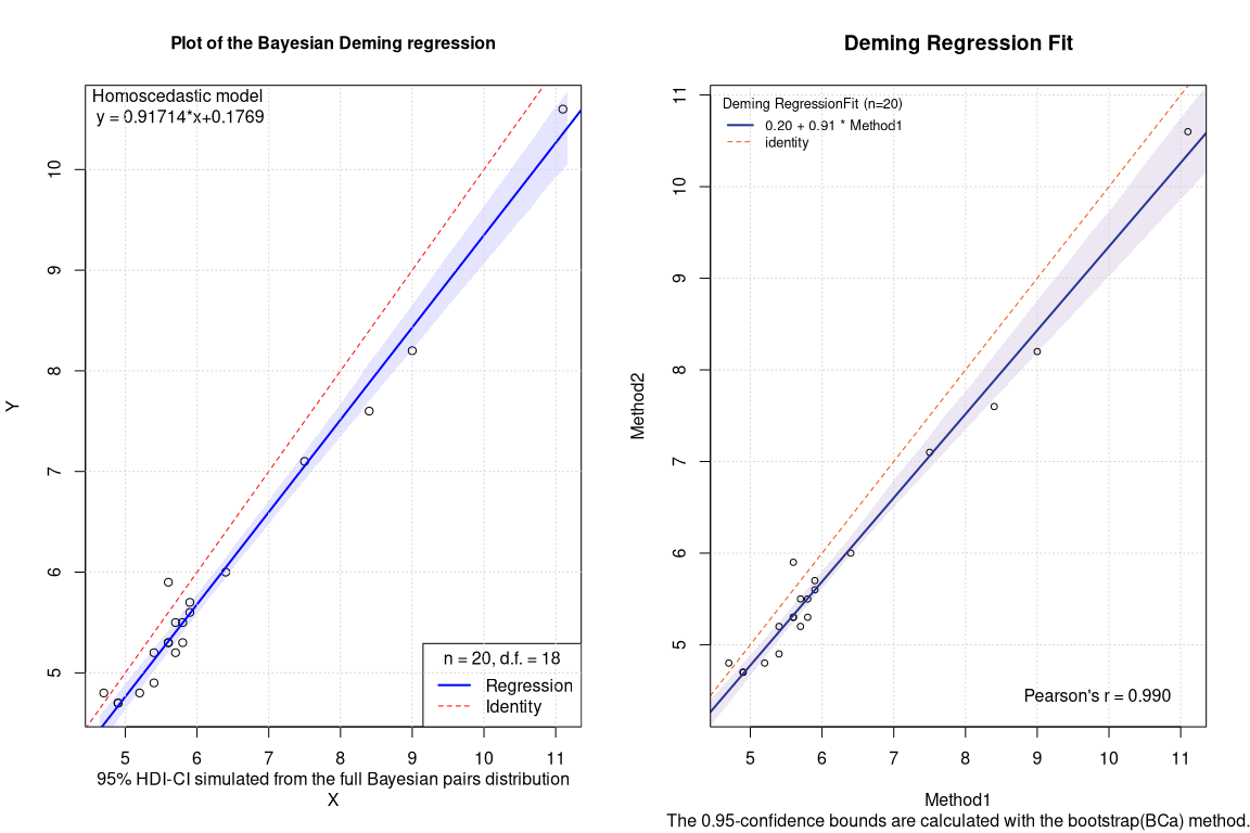
Frequentist Deming bootstrapped BCa CI

##                 EST SE        LCI       UCI
## Intercept 0.2035609 NA -0.2936662 0.6669625
## Slope     0.9142874 NA  0.8355696 1.0012592

Bayesian Deming- CI

## Inference for Stan model: bdpreg_homotrunc.
## 4 chains, each with iter=2000; warmup=1000; thin=1; 
## post-warmup draws per chain=1000, total post-warmup draws=4000.
## 
##              mean se_mean     sd    2.5%     25%     50%     75%   97.5% n_eff
## intercept  0.1769  0.0073 0.2229 -0.2773  0.0360  0.1765  0.3252  0.6179   922
## slope      0.9171  0.0012 0.0353  0.8479  0.8945  0.9173  0.9393  0.9897   928
## sigma      0.1571  0.0008 0.0306  0.1089  0.1355  0.1533  0.1745  0.2308  1493
## lp__      24.9337  0.0413 1.3201 21.4045 24.2905 25.2901 25.9177 26.4503  1023
##             Rhat
## intercept 1.0027
## slope     1.0030
## sigma     1.0024
## lp__      1.0044
## 
## Samples were drawn using NUTS(diag_e) at Mon Mar  4 22:52:39 2024.
## For each parameter, n_eff is a crude measure of effective sample size,
## and Rhat is the potential scale reduction factor on split chains (at 
## convergence, Rhat=1).

The differences in the coefficients are rather minimal. By contrast, in this case, the confidence intervals of the Bayesian regression seem slightly less conservative.

Robust Bayesian Deming vs equivariant (bootstrapped BCa) Passing Bablok

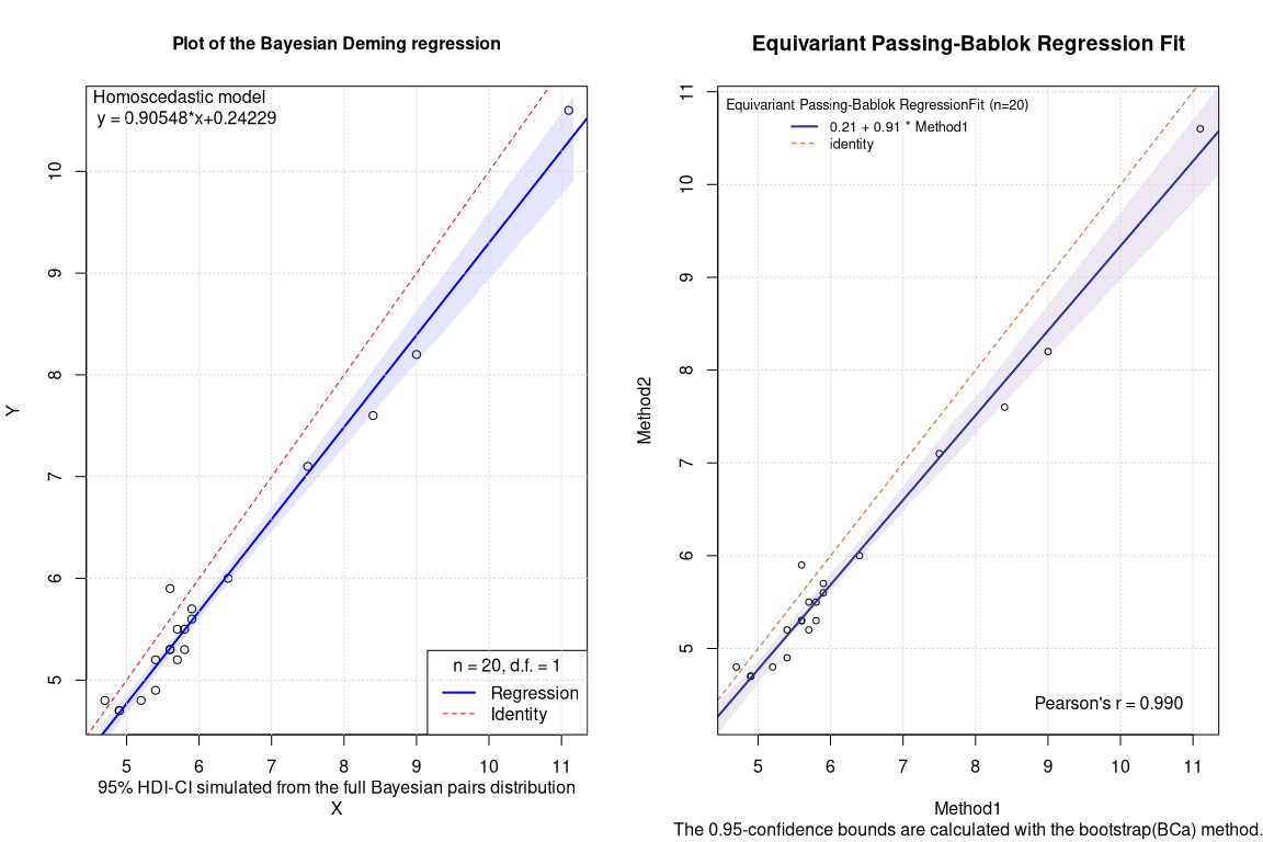
Frequentist PBequi bootstrapped BCa CI

##                 EST SE        LCI       UCI
## Intercept 0.2097009 NA -0.3500000 0.7042857
## Slope     0.9128716 NA  0.8285714 1.0000000

Bayesian Deming robust regression CI (df=1):

## Inference for Stan model: bdpreg_homotrunc.
## 4 chains, each with iter=2000; warmup=1000; thin=1; 
## post-warmup draws per chain=1000, total post-warmup draws=4000.
## 
##              mean se_mean     sd    2.5%     25%     50%     75%   97.5% n_eff
## intercept  0.2423  0.0103 0.2644 -0.1998  0.0318  0.2254  0.4554  0.7214   664
## slope      0.9055  0.0018 0.0457  0.8231  0.8667  0.9094  0.9435  0.9779   653
## sigma      0.0800  0.0007 0.0269  0.0380  0.0612  0.0760  0.0947  0.1438  1404
## lp__      27.7885  0.0394 1.2998 24.3188 27.2930 28.1701 28.6811 29.1170  1090
##             Rhat
## intercept 1.0042
## slope     1.0042
## sigma     1.0019
## lp__      1.0033
## 
## Samples were drawn using NUTS(diag_e) at Mon Mar  4 22:52:47 2024.
## For each parameter, n_eff is a crude measure of effective sample size,
## and Rhat is the potential scale reduction factor on split chains (at 
## convergence, Rhat=1).

When comparing the robust methods, the most striking thing is that the confidence intervals of the PBequi regression show a suspicious integer value of 1 as the upper limit of the slope. This phenomenon is similar to what was reported in 2021 on arxiv. The 2D box ellipses (BE) plot of the bootstrapped pairs can elucidate the situation.

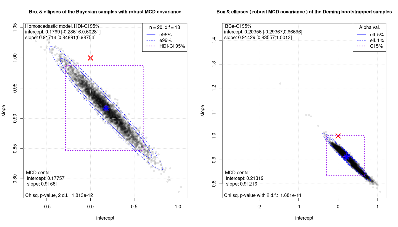
Box Ellipses plots: the non robust Deming regressions

Box Ellipses plots: the robust methods

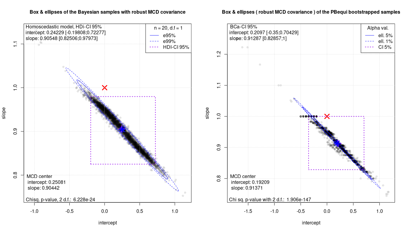
In general Bayesian sampling looks smoother. It is also noticeable that for the Passing Bablok equivariant regression, the bootstrap pair plot shows the same accumulation phenomena as reported in 2021. This also explains the suspicious value noted for the slope confidence intervals.

The Mahalanobis distance testing is in all cases much more powerful. The equivalence of the two methods can be safely rejected with just 20 samples. At the same time the 2D plot also offers an insight into the quality of the regressions and of the data. This is especially worth for bootstrapped methods. Clearly PBequi combined with bootstrap shows a far from ideal BE plot.

Analytical equivariant Passing Bablock

It is also worth comparing the bootstrap confidence intervals with the analytical ones for the PBequi method.

##                 EST         SE        LCI       UCI
## Intercept 0.2097009 0.23933930 -0.2931323 0.7125341
## Slope     0.9128716 0.04249835  0.8235859 1.0021574

The confidence intervals are coherent and larger that those from the robust Bayesian method.

Remark: The {rstanbdp} library used here is the devel version available on github. It has some graphical differences/improvements. It is available with install_github(“piodag/rstanbdp/tree/devel”)