Abstract

Method validation is particularly challenging when data shows strong heteroscedasticity. It is very hard to distinguish outliers, especially in the high range of values where variance is larger. Here a Bayesian Deming regression approach with a linear heteroscedastic model from the {rstabdp} package is applied to a collection of tireoglobuline measurements¹. This innovative model is found very reliable. The analysis of the standardized residuals shows that each point contributes in a balanced manner to the determination of the coefficients and confidence intervals. Bayesian homoscedastic Deming and classical frequentist Deming regression offer similar results. Linear heteroscedastic Bayesian Deming regression, on the other hand, offers similar results to Passing Bablok equivariant regression. Finally, the robustification of the linear heteroscedastic model is also carried out, without, however, finding values that differ greatly from the non-robust version. In this case, once the error structure is corrected, there is no more data with sufficient leverage to alter the result of the non-robust regression from the robust one.

Tireoglobuline data set

The distribution of tireoglobuline samples (n = 139 pairs) is far from ideal. Most values are at very low concentration and very few data points shows very high concentrations. The total range is [0.194;4220] for the Method1 and [0.206;3562] for Method2. The medians are 1.530 and 1.267 showing an extreme distribution asymmetry. Under these circumstances is very hard to offer a proper graphical representation of the distributions. Thus we just report here a row of quantiles.

##       10%       25%       50%       75%       90%       95%       99% 
##    0.4060    0.6165    1.5300    5.2800   37.7100  263.7500 3174.4600

##       10%       25%       50%       75%       90%       95%       99% 
##    0.3568    0.5165    1.2670    4.0500   28.1190  142.1497 2704.6576

Linear heteroscedastic model vs homoscedastic model

The results for the method comparison between an homoscedastic and a linear heteroscedastic Bayesian model are reported below. The homoscedastic model is strongly influenced by the few values at very high concentration. The heteroscedastic model, on the other hand, is able to balance the errors as a function of the measured concentrations and thus all points contribute in a similar manner.

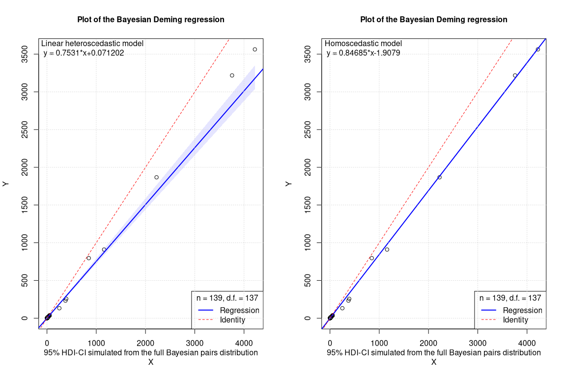
The plot with the confidence intervals shows that in the case of the homoscedastic model (on right side), the variance is largely underestimated especially at high concentrations. The two slopes are completely different but this comes as no surprise since in the homoscedastic model the largest part of the data at low concentrations is simply neglected.

The comparison of the standardized residual plots is striking. To perform this at best it is necessary to print a second TA plot zooming into the low concentration data range (second row of the plot).

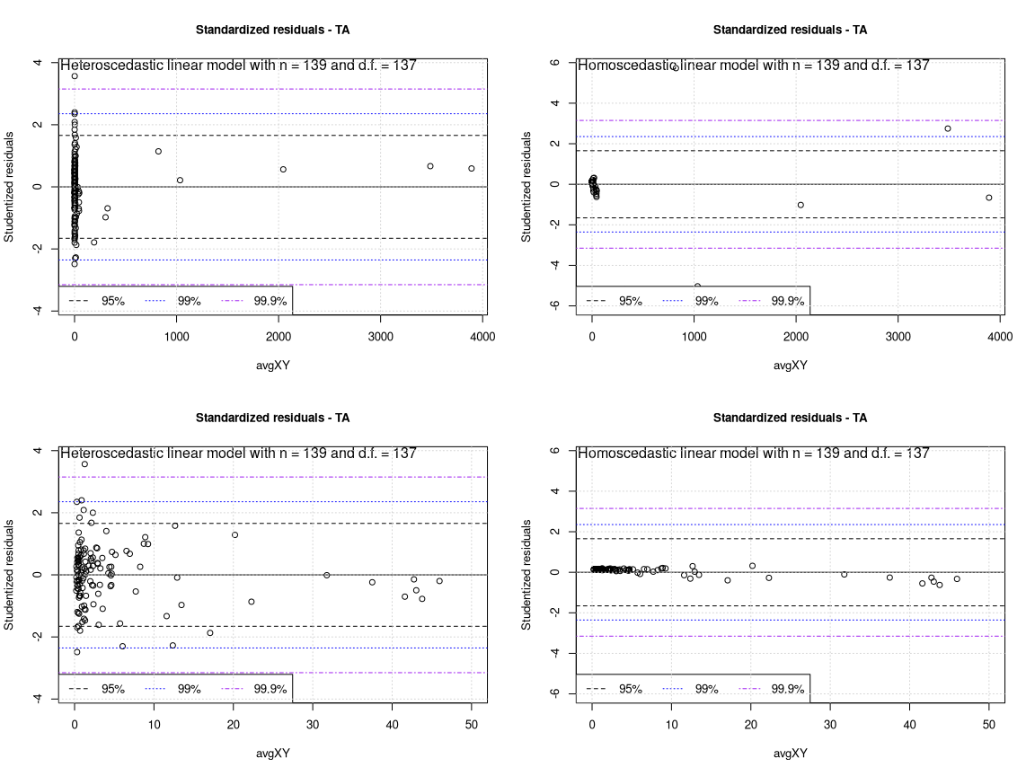
With the linear heteroscedastic model all data points contribute to the regression in a balanced way. The TA plots on the left show an elegant band of residuals and this band is confirmed also in the zoomed in figure. Only a single weak outlier may be present at very low concentrations.

In the homoscedastic model on the right the variance of the majority of the points is nearly zero and only very few points effectively contribute to the global error and thus to the parameters estimation.

Comparison with equivariant Passing Bablok regression and frequentist Deming regression

Here below the plots for Deming and equivariant Passing Bablok regressions from {mcr} package.

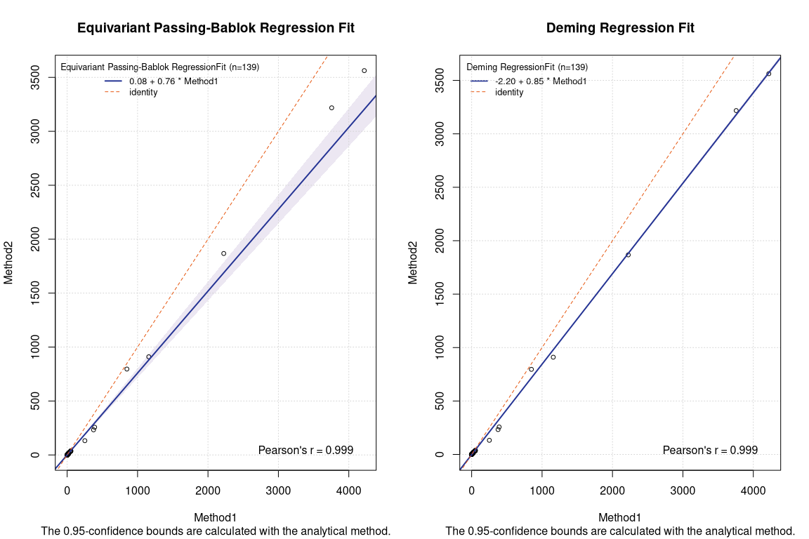
The results are in line with the expectations. Frequentist Deming regression and Bayesian Deming regression show very similar results. The robust equivariant Passing Bablok regression provides a result very similar the linear heteroscedastic Bayesian Deming regression.

Confidence intervals comparison

Linear heteroscedastic Bayesian model vs equivariant Passing Bablok

## Inference for Stan model: bdpreg_linhettrunc.
## 4 chains, each with iter=2000; warmup=1000; thin=1; 
## post-warmup draws per chain=1000, total post-warmup draws=4000.
## 
##              mean se_mean     sd    2.5%     25%     50%     75%   97.5% n_eff
## intercept  0.0712  0.0004 0.0156  0.0407  0.0610  0.0713  0.0815  0.1020  1954
## slope      0.7531  0.0004 0.0187  0.7167  0.7402  0.7525  0.7655  0.7914  2101
## Alpha      0.0146  0.0002 0.0089  0.0012  0.0078  0.0133  0.0199  0.0349  1973
## Beta       0.1334  0.0003 0.0114  0.1123  0.1255  0.1332  0.1410  0.1566  1549
## lp__      71.5848  0.0477 1.5225 67.7420 70.8610 71.9235 72.6755 73.5034  1020
##             Rhat
## intercept 1.0002
## slope     1.0001
## Alpha     1.0002
## Beta      1.0007
## lp__      1.0028
## 
## Samples were drawn using NUTS(diag_e) at Sat Mar 23 23:02:28 2024.
## For each parameter, n_eff is a crude measure of effective sample size,
## and Rhat is the potential scale reduction factor on split chains (at 
## convergence, Rhat=1).

##                  EST         SE        LCI       UCI
## Intercept 0.07638151 0.01780703 0.04116933 0.1115937
## Slope     0.75924658 0.02226690 0.71521532 0.8032778

Equivariant Passing Bablok coefficients and CI are very similar to the linear heteroscedastic Bayesian Deming ones. The Bayesian method seems slightly less conservative. It is possible that the better error management of the linear heteroscedastic method leads to an intrinsic higher power of the method. It has been reported that classic method comparison methods like Deming and classic Passing Bablok tend to lose power lose power with heteroscedastic data.

Homoscedastic Bayesian vs classical frequentist Deming model

## Inference for Stan model: bdpreg_homotrunc.
## 4 chains, each with iter=2000; warmup=1000; thin=1; 
## post-warmup draws per chain=1000, total post-warmup draws=4000.
## 
##                mean se_mean     sd      2.5%       25%       50%       75%
## intercept   -1.9079  0.0232 1.1800   -4.1846   -2.7079   -1.9179   -1.1330
## slope        0.8469  0.0000 0.0024    0.8422    0.8452    0.8468    0.8485
## sigma       10.5771  0.0137 0.7025    9.3364   10.0722   10.5377   11.0279
## lp__      -406.3100  0.0296 1.2413 -409.4606 -406.8678 -406.0010 -405.4306
##               97.5% n_eff   Rhat
## intercept    0.3596  2587 1.0001
## slope        0.8515  5092 0.9993
## sigma       12.0495  2626 1.0005
## lp__      -404.9119  1753 1.0029
## 
## Samples were drawn using NUTS(diag_e) at Sat Mar 23 23:02:35 2024.
## For each parameter, n_eff is a crude measure of effective sample size,
## and Rhat is the potential scale reduction factor on split chains (at 
## convergence, Rhat=1).

##                  EST          SE        LCI       UCI
## Intercept -2.2027208 1.319133325 -4.8112162 0.4057746
## Slope      0.8468267 0.002480548  0.8419216 0.8517318

Frequentist and Bayesian homoscedastic coefficients and CI are are also very similar. They are in both cases really to narrow. This is the consequence of the bad error management.

Robustification of the Bayesian regressions

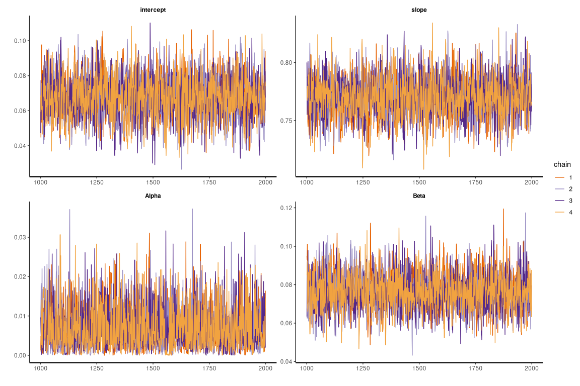
With the Bayesian Deming regression the robustification of models can be applied in a very simple way, decreasing the degree of freedom (df) of the T distributed sampled residuals. Here the regression is run with maximal robustness, at df=1.

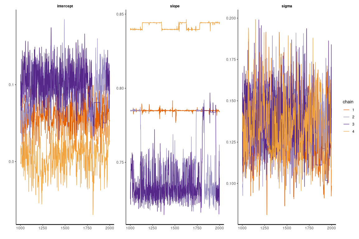
Here the traceplot for the linear heteroscedastic model

Unfortunately in this case it was not possible to get a good convergence of the sampling with the homoscedastic model at df=1 (and in general at low df values). Here below an example of a non converging traceplot. It can be assumed that there are conflicting trends between the regression parameters promoted by data at low concentrations and by data at high concentrations.

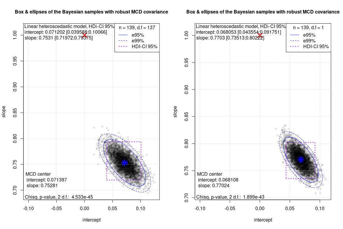
The differences between the robust and the non robust linear heteroscedastic Bayesian model are rather small. The reason behind could be that, once the heteroscedasticity is managed, there are no strong leveraged outliers left that can significantly alter the regression.

Here below the two Box Ellipses plot for the comparison between the robust and the non robust linear heteroscedastic models

Conclusions

The linear heteroscedastic model provides a very convenient method to perform method comparison analysis on heteroscedastic data. In most cases there is no need to robustify the regression although this is possible and easy. The heteroscedastic management of the variance can accommodate the data in a correct way and the end result looks very organic and is easy to be checked via the standardized residual plot. Moreover, it has been previously reported that Passing Bablok methods are subject to bias. Thus, a model with an appropriated error structure should be preferred to a potentially biased one.

Worth mentioning is that the Bayesian Deming regression can be also performed with moderate robustification, running for example the regression at df = 5 and providing some approximated 3 sigma additional tolerance for the residuals, as reported by different authors like A. Gelman.